Author: Olzhas S. Tazabekov (LinkedIn)
Prerequisites: basic programming skills with Python and SPICE
Intro: Why is All the Buzz
Throughout our University degree programs, we all learned how to analyze, design and verify electrical circuits. Unfortunately or fortunately, most of us were trained using industry level graded software (e.g. Cadence, Synopsys, etc.). However, in real life (outside of school) that software does come with a pretty heavy price associated with the cost of licenses and IT infrastructure. So, unless you are heavy weight semiconductor giant with millions in corporate accounts it is a quite a challenge to afford. Where does this leave all those half starving tech startups or ordinary people? Open source software has been one of the answers so far (another one is to sell a kidney of one of the board members and purchase an IC design tool license 😉 ).
PySpice
A while ago I stumbled across PySpice, a library for python 3, that interplays with a SPICE simulator (ngspice to be precise). Even though it lacks a graphical user interface and schematic capture editor, hence, one can’t simply go drag-n-dropping elements or click-n-plotting waveforms the old school way, it does come with a support of powerful high-level object-oriented Python 3 which is perfectly suited for working with circuits and scientific framework like Numpy and Matplotlib which is great for data processing, analysis and visualization.
All the documentation and installation guidelines can be found here:
https://pypi.python.org/pypi/PySpice/0.3.3
For those who are new with SPICE or Python, there is a pretty well written set of examples explaining how to get started with simple circuits and basic analysis and data processing.
https://pyspice.fabrice-salvaire.fr/examples/index.html
Ideal DAC
This section explains how to develop a model for ideal Digital-to-Analog Converter which could be later plugged into a more complex mixed signal model. Our goal is to make use of convenience of python object oriented programming and power of data processing framework.
There are an infinite number of ways to implement a model of an ideal DAC. Before we move on to the code let’s review some DAC basics.
Along with input code, supply/ground and output pins the most simple DAC block usually have two reference voltages, Vref+ and Vref- assuming Vref+>Vref-. When a digital input is at the smallest possible number, the DAC output voltage becomes Vref-. When the input code number is increased by one, the output of the DAC (an analog voltage defined at discrete amplitude levels) increases by least significant bit (LSB). Therefore, we have 1LSB = (Vref+ – Vref-)/2^N, where N is a number of bits for the input code. We will be assuming that the DAC output ranges from Vref- up to Vref+ – 1LSB. We could just as easily have assumed the output ranging from Vref- + 1LSB up to Vref+. The important thing is to notice that the DAC output range is 1LSB smaller than Vref+ – Vref-. If one needs more resolution the one can simply increase the number of bits, N, used and hence decrease the value of the DAC’s LSB.
One can write the DAC output in terms of reference voltages and digital codes bn (i.e. logic 0 and 1). Assuming, bn = 0 for all the codes Vout is equal to Vref-. Then,
![\[ V_{out} =1/2^N (V_{ref+}-V_{ref-})(b_{N-1}2^{N-1}+b_{N-2}2^{N-2}+...+b_0)+V_{ref-}) \]](http://www.tazabekov.com/blog/wp-content/ql-cache/quicklatex.com-3a7175ba9dee43ff2d888c0ac742d3c2_l3.png "Rendered by QuickLaTeX.com")
This can be implemented using nonlinear dependent source.
self.voltage_expression = ''.join(['(v(refp)-v(refn))/'+str(2**self.nbits)+'*(']+[('v(b'+str(i)+'l)*'+str(2**i)+'+') for i in range(self.nbits)]+['0)+v(refn)'])
self.BehavioralSource('out', 'out', 'vss', voltage_expression=self.voltage_excolpression)
voltage_expression is a string, which defines the output voltage value depending on the number of bits and reference voltages. Then this string gets passed as a parameter to a BehavioralSource.
PySpice Modelling Approach
As was mentioned earlier, Python is a powerful high level language that gives you a great level of freedom and flexibility implementing things in object oriented way. SPICE most commonly deals with circuits, subcircuits and elements.
Previous section described what is needed to implement an ideal DAC (e.g. trip voltage generating resistive divider, Bit logic elements and behavioral source). In the following implementation the bit logic elements with the resistive divider will be a separate subcircuit inside a DAC subcircuit. The top level circuit is usually a test bench used for characterization.
Below is a diagram of how to structure your test benches. Now, most IC design engineers are familiar with SPICE and concept of netlist, circuits, subcircuits, etc. However, things can get confusing when one tries to transition from SPICE paradigm into a Object-Oriented Programming paradigm.

Fig. 1. Object-Oriented Mapping from SPICE circuits (Left) to Python classes (Right)
PySpice has Spice.Netlist namespace with Circuit and SubCircuitFactory generic classes, which can be used to create classes for your own circuits and subcircuits. Let’s move on to an example. The following code creates a class of BitLogic element, which generates a solid logic level, i.e. an input logic code would assumed to be a valid logic “1” if its amplitude is greater than VDD/2 and a logic “0” if its amplitude is less than VDD/2.
'''
BitLogic Subcircuit Schematic

    vdd
     |
bx--\----trip
     |
     |---bxl
     |
bx----/--trip
     |
    vss

Trip V generation Schematic

    vdd
     |
   |res|
     |---trip
   |res|
     |
    vss

'''
class BitLogic(SubCircuitFactory):
    __name__='BITLOGIC' # subcircuit name
    __nodes__=('bx', 'bxl', 'vdd', 'vss') # subcircuit nodes set
    def __init__(self):
        super().__init__() # initialize a parent class - SubCircuitFactory
        # add model parameters for the ideal switches to the BitLogic Subcircuit
        self.swmod_params = {'ron':0.1, 'roff':1E6}
        self.model('swmod','sw', **self.swmod_params)
        # add a resistive voltage divider to generate the threshold voltage value for switching
        self.R('top', 'vdd', 'trip', 100E6)
        self.R('bot', 'trip', 'vss', 100E6)
        # add swicthes and specify their model parameters
        self.VCS('top', 'bx', 'trip', 'vdd', 'bxl', model='swmod')
        self.VCS('bot', 'trip', 'bx', 'bxl', 'vss', model='swmod')
The netlist will be generated by PySpice when one makes an instance of this Class. The cool thing about this approach is that one can configure the objects (hence, subcircuit netlists) by any means available through the Class methods. On top of that, complex systems can be implemented via incorporating basic subcircuit Class instances into other bigger instances. A DAC subsircuit Class would be a good example of that.
'''
Ideal DAC SubCircuit Shematic
     refp vdd
      |    |
     --------------------------------------
b0--| |bitlogic0|--bxl0--|              |  |
b1--| |bitlogic1|--bxl1--|  behavioral  |--|--out
... | ...                |voltage source|  |
b5--| |bitlogic5|--bxl5--|              |  |
     --------------------------------------
      |    |
     refn vss
'''
class IdealDac(SubCircuitFactory):
    __name__ = 'IDEALDAC'
    def __init__(self, nbits, **kwargs):
        # number of bits passed as a parameter
        self.nbits = nbits
        # nodes definition based on nbits parameter
        self.__nodes__ = ('refp', 'refn', 'vdd', 'vss') + tuple([('b'+str(i)) for i in range(self.nbits)]) + ('out',)
        super().__init__()
        # add an nbit number of BitLogic subcircuits
        for i in range(0, self.nbits):
            bitstr = str(i)
            self.X('BL'+bitstr, 'BITLOGIC', 'b'+bitstr, 'b'+bitstr+'l', 'vdd', 'vss')
        # make an output voltage expression based on nbits parameter and pass this string into added BehavioralSource
        self.voltage_expression = ''.join(['(v(refp)-v(refn))/'+str(2**self.nbits)+'*(']+[('v(b'+str(i)+'l)*'+str(2**i)+'+') for i in range(self.nbits)]+['0)+v(refn)'])
        self.BehavioralSource('out', 'out', 'vss', voltage_expression=self.voltage_expression)
Now, all that’s left is to make the Test Bench instance of class Circuit, connect instances of the subcircuit classes, specify analysis one needs to run, extract and post process the data.
The following example runs an operating point analysis for 4 bit DAC and prints voltages for all the nodes in the testbench.
if __name__ == "__main__":
    dac_nbits=4 # specify a number of bits for the DAC
    # operating point analysis
    circuit_op = Circuit('DAC_TestBench') # add an instance of class Circuit to be your testbench
    circuit_op.subcircuit(BitLogic()) # add an instance of BitLogic Subcircuit
    circuit_op.subcircuit(IdealDac(nbits=dac_nbits)) # add an instance of DAC Subcircuit
    circuit_op.X('DAC1', 'IDEALDAC', 'vrefp', 'vrefn', 'vdd', 'vss', ','.join([('b'+str(i)) for i in range(dac_nbits)]), 'out') # connect the DAC subcircuit into the testbench
    circuit_op.V('vdd', 'vdd', circuit_op.gnd, 1) # connect VDD voltage source to vdd node of the DAC subcircuit
    circuit_op.V('vss', 'vss', circuit_op.gnd, 0) # connect VSS voltage source to the ground node of the DAC subcircuit
    circuit_op.V('refp', 'vrefp', circuit_op.gnd, 1) # connect positive reference voltage source to the vrefp node of the DAC subcircuit
    circuit_op.V('refn', 'vrefn', circuit_op.gnd, 0) # connect negative reference voltage source to the vrefn node of the DAC subcircuit
    for i in range(dac_nbits):
        istr=str(i)
        circuit_op.V('b'+istr, 'b'+istr, circuit_op.gnd, 1) # connect nbit number of voltage sources to provide the input code (all '1's in this case)
    simulator_op = circuit_op.simulator(temperature=25, nominal_temperature=25) # add simulator conditions (e.g. temperature)
    analysis_op = simulator_op.operating_point() # specify the analysis to be an operating point analysis
    for node in analysis_op.nodes.values():
        print('Node {}:{:5.2f} V'.format(str(node),float(node))) # print voltage values of all the nodes of the tesbench
The results confirm that an input code of ‘1111’ gives an output voltage of 0.94V. One may configure an input code differently and get the desired output voltage.
Node vdd [voltage]: 1.00 V
Node xdac1.xbl0.trip [voltage]: 0.50 V
Node vss [voltage]: 0.00 V
Node xdac1.b0l [voltage]: 1.00 V
Node b0 [voltage]: 1.00 V
Node xdac1.xbl1.trip [voltage]: 0.50 V
Node xdac1.b1l [voltage]: 1.00 V
Node b1 [voltage]: 1.00 V
Node xdac1.xbl2.trip [voltage]: 0.50 V
Node xdac1.b2l [voltage]: 1.00 V
Node b2 [voltage]: 1.00 V
Node xdac1.xbl3.trip [voltage]: 0.50 V
Node xdac1.b3l [voltage]: 1.00 V
Node b3 [voltage]: 1.00 V
Node out [voltage]: 0.94 V
Node vrefp [voltage]: 1.00 V
Node vrefn [voltage]: 0.00 V
However, one might as well also make use of flexibility provided by Python and print output voltages for all the corresponding input codes. On top of that, there are numerous tools available in Python for data post processing and graphic visualization.
So, the next example shows how to run a series of operating point analysis to calculate the DAC output voltage for each input code and plot its transfer function.
    # DAC transfer function - outut voltage vs input code test bench based on operating point analysis
    input_codes = np.arange(2**dac_nbits)
    bin_input_codes = np.zeros(2**dac_nbits)
    outputs = np.zeros(2**dac_nbits)
    for number in input_codes:
        circuit_tf = Circuit('DAC Transfer Function')
        circuit_tf.subcircuit(BitLogic())
        circuit_tf.subcircuit(IdealDac(nbits=dac_nbits))
        circuit_tf.X('DAC1', 'IDEALDAC', 'vrefp', 'vrefn', 'vdd', 'vss', ', '.join([('b'+str(i)) for i in range(dac_nbits)]), 'out')
        print(', '.join([('b'+str(i)) for i in range(dac_nbits)]))
        circuit_tf.V('vdd', 'vdd', circuit_tf.gnd, 1)
        circuit_tf.V('vss', 'vss', circuit_tf.gnd, 0)
        circuit_tf.V('refp', 'vrefp', circuit_tf.gnd, 1)
        circuit_tf.V('refn', 'vrefn', circuit_tf.gnd, 0)
        num_bin_array = [int(num) for num in list(format(number, '0'+str(dac_nbits)+'b'))]
        rev_num_bin_array = list(reversed(num_bin_array))
        for i in range(dac_nbits):
            istr=str(i)
            circuit_tf.V('b'+istr, 'b'+istr, circuit_tf.gnd, 1*rev_num_bin_array[i])
        simulator_tf = circuit_tf.simulator(temperature=25, nominal_temperature=25)
        analysis_tf = simulator_tf.operating_point()
        outputs[number] = float(analysis_tf.nodes['out'])
        print('number: {} - output: {:5.3f}'.format(str(num_bin_array), outputs[number]))
    plt.title(circuit_tf.title)
    plt.xlabel('Input Code')
    plt.ylabel('DAC Output Voltage [V]')
    bin_input_codes = [format(code, '0'+str(dac_nbits)+'b') for code in input_codes]
    plt.xticks(input_codes, bin_input_codes, rotation='vertical')
    plt.plot(input_codes, outputs, 'r--')
    plt.plot(input_codes, outputs, 'ko')
    plt.grid()
    plt.show()
The “input code – output voltage” table and the transfer function plot will look as follows
number: [0, 0, 0] - output: 0.000
b0, b1, b2
number: [0, 0, 1] - output: 0.125
b0, b1, b2
number: [0, 1, 0] - output: 0.250
b0, b1, b2
number: [0, 1, 1] - output: 0.375
b0, b1, b2
number: [1, 0, 0] - output: 0.500
b0, b1, b2
number: [1, 0, 1] - output: 0.625
b0, b1, b2
number: [1, 1, 0] - output: 0.750
b0, b1, b2
number: [1, 1, 1] - output: 0.875
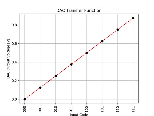
Fig. 2. Transfer Function of 3 bits DAC
Even though “scripting” the circuits might look like a bit of taking the scenic route to the results while compared to drag-n-dropping the elements with mouse. The approach has its own advantages. Once properly written, verified and documented, one may re-use them and pass it to other people with no complications making the approach ideal for team development and regression testing.
For example, the code above can be easily modified to change the number of bits or reference voltages.

Fig. 3. Transfer Function of 5 bits DAC with Positive Reference of 1 V
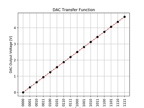
Fig. 4. Transfer Function of 4 bits DAC with Positive Reference of 5 V
Conclusions
This tutorial explains how to model a digital to analog converter with PySpice. It is definitely a cool tool for people interested in programming and circuits. Of course, industry graded spice simulators are probably a way more advanced compared to ngspice. On top of that, PySpice doesn’t offer a graphic user interface and drag-n-drop approach. However, it does come with a support of powerful object-oriented Python3 and scientific frameworks, which are great for data post-processing, analysis and visualization.
General References
- GitHub Repository with the complete code for this tutorial: https://github.com/OlzhasT/PySpiceCircuits-/blob/master/dac_ideal_subcircuit_class_test.py,
- All the PySpice documentation and installation guidelines: https://pypi.python.org/pypi/PySpice/0.3.3,
- PySpice examples explaining how to get started with simple circuits and basic analysis and data processing: https://pyspice.fabrice-salvaire.fr/examples/index.html;
I’d like to thank Matthew James (LinkedIn) for his contribution to this article.